Indexed Simplex Set Package
Mesh Functions
The functions which operate on indexed simplex sets are categorized as follows:
- Accessors
- Builders
- Build from simplices.
- Boundary condition functions for simplicial meshes.
- CellAttributes
- Identify distinct points and remove duplicate points.
- Equality
- File I/O for IndSimpSet
- Fit a mesh to a level-set description.
- Geometric functions for simplicial meshes.
- Laplacian Smoothing
- Vertices on a manifold
- Optimization
- Quality
- Set Operations
- Laplacian Smoothing with a Solve
- Subdivision for IndSimpSet
- Tiling
- Topology Functions for IndSimpSet
- Transfer Fields
- Transform Vertices or Simplices
Mesh Data Structures
geom::IndSimpSet implements an indexed simplex set. It is composed of an array of vertices and an array of indexed simplices. Below is a mesh of the unit square. The vertex indices are labelled outside the square. The indices inside indicate the order of the vertices for the three triangles.
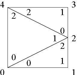
A mesh of the unit square.
  0.0 0.0
  1.0 0.0
  1.0 0.5
  1.0 1.0
  0.0 1.0
and an array of indexed simplices.
  0 1 2
  0 2 4
  2 3 4
The geom::IndSimpSetIncAdj class inherits from geom::IndSimpSet and stores additional topological information. It uses geom::VertexSimplexInc to store vertex-simplex incidences and geom::SimplexAdj to store simplex adjacencies. Geometric mesh optimization capabilities are implemented using this augmented data structure.
For the above unit square, the vertex-simplex incidences are:
  0 1
  0
  0 1 2
  2
  1 2
These are stored in a packed array. The simplex adjacencies are represented as:
  -1 1  -1
  2  -1 0
  -1 1  -1
where -1 indicates no adacent neighbor. For example, triangle 0 has no adjacent neighbors opposite its first and third vertices and has triangle 1 opposite its second vertex.
Consider an (N-1)-D manifold  in N-D space (perhaps a curve in 2-D or a surface in 3-D.) The manifold can be described explicitly or implicitly. An explicit description could be parametric. For example, the unit circle is:
![\[ \{ (x,y) : x = \cos(\theta), y = \sin(\theta), 0 \leq \theta < 2 \pi \} \]](form_151.png)
A simplicial mesh is also an explicit description of a manifold.
For some purposes an implicit description of a manifold is more useful. One common implicit representation is a level set function. For example, the unit circle is the set of points on which the function  is zero. This level set function is useful for determining if a point is inside or outside the circle. If
  is negative/positive then the point
  is inside/outside the circle.
One special kind of level set function is a signed distance function.  is a signed distance function for the unit cirle. That is, the value of the function is the distance to the circle. The distance is negative inside the circle and positive outside.
A related concept is a closest point function. As the name suggests, the function evaluates to the closest point on the manifold. For the unit circle, the closest point function is
![\[ c(x,y) = \frac{(x,y)}{ \sqrt{x^2+y^2} } \ \mathrm{ for }\ (x,y) \neq (0,0) \]](form_156.png)
![\[ c(x,y) = (1,0) \ \mathrm{for}\ (x,y) = (0,0) \]](form_157.png)
(Note that the closest point is not uniquely determined for  .)
.)
Consider a manifold that is the boundary of an object. A distance function for the manifold can be used to determine if a point is inside or outside the object. Or it can be used to determine if a point is close the boundary of the object. The closest point function is useful if points need to be moved onto the boundary.
The geom::ISS_SignedDistance class computes the distance to a simplicial mesh and the closest point on the simplicial mesh. It stores the simplices is a bounding box tree. It efficiently computes distance and closest point by using a technique called a lower/upper bound query. This class is used both in mesh generation and in geometric optimization of boundary vertices.
Use the indexed simplex set classes by including the file geom/mesh/iss.h or by including geom/mesh.h .
Mesh Quality
We assess the quality of a mesh in terms of the quality of its elements. The  norm of the quality metric over all tetrahedra gives the quality of the mesh. We can use the
  norm to obtain an average quality or the
  norm to measure the worst element quality.
The operations we apply to optimize the mesh are local. They only affect the complex of tetrahedra which are adjacent to a node, edge or face. We use the norm to measure the quality of the complex.
Geometric Optimization of a Node Location
The tetrahedra adjacent to an interior vertex  form a complex. We move to optimize the norm of the quality metrics of the simplices in the complex.
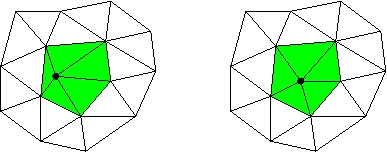
2-D illustration. The complex is shown in green.
We have investigated using optimization methods that do not require derivative information. These have the advantage that one can optimize the (max norm) of the quality metric. We implemented the downhill simplex method and the coordinate descent method. However, we have found that optimizing the norm with a quasi-Newton method (BFGS) is more robust and much more efficient.
Geometric Optimization of Boundary Nodes
For impact/penetration problems, the greatest deformation occurs at the boundary. It is not possible to arrange the interior nodes to obtain a quality mesh if the boundary nodes have poor geometry. Thus we extended the geometric optimization to boundary nodes.
One approach is to optimize the position of the boundary node and then project it onto the boundary curve/surface. We use an implicit representation of the boundary. The projection is done with the closest point function.
Boundary node optimization subject to a surface constraint.
Constant Content Constraint
Another approach is to conserve the content (volume in 3-D) of the complex of simplices adjacent to the boundary node. This is easy to implement and conserves mass. We use a penalty method combined with a quasi-Newton optimization. (We use the same optimization method as for interior nodes. Only the objective function changes by adding a penalty.)

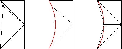
Boundary node optimization subject to a constant volume constraint.
A boundary node should be moved only if the surface is approximately planar at the node. In the first example, the surface at the boundary node is planar. Thus the boundary shape is unchanged. In the second example, there is a large difference between the adjacent boundary edge normals. This leads to a large change in the shape of the boundary.
Geometric Optimization
The user chooses the movable set of nodes. They may choose all or a subset of the interior or boundary nodes. The user may use the condition number or mean ration metrics or supply their own metric.
We have implemented several hill climbing methods for sweeping over the nodes of the mesh. One can sweep over all movable nodes. Or one can sweep over movable nodes that have an adjacent tetrahedron with poor quality.
These hill climbing methods apply local changes to the mesh. They rapidly improve deformations that are local in nature. It may take many iterations to converge if the nodes are widely re-distributed.
Generated on Thu Jun 30 02:14:58 2016 for Computational Geometry Package by
 1.6.3
1.6.3