A Survey of Different Boundary Conditions in Geometric Optimization of the Enterprise Mesh.

Here we apply geometric optimization to a mesh using a variety of boundary constraints. We start with a mesh of the Enterprise that has 1,438 nodes and 4,926 elements. (The following commands can be executed in stlib/examples/geom/mesh. The stlib/results/geom/mesh/3/enterpriseBoundarySurvey directory contains a makefile which generates the figures in this example.)

  cp ../../../data/geom/mesh/33/enterpriseL50.txt enterprise.txt 

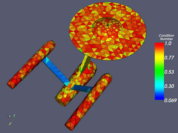
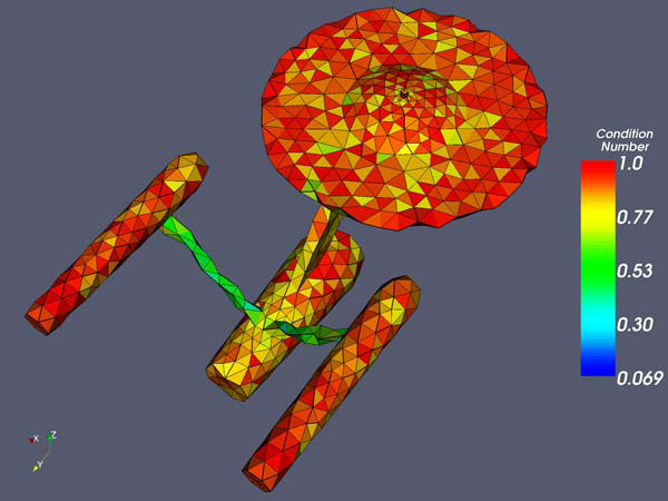
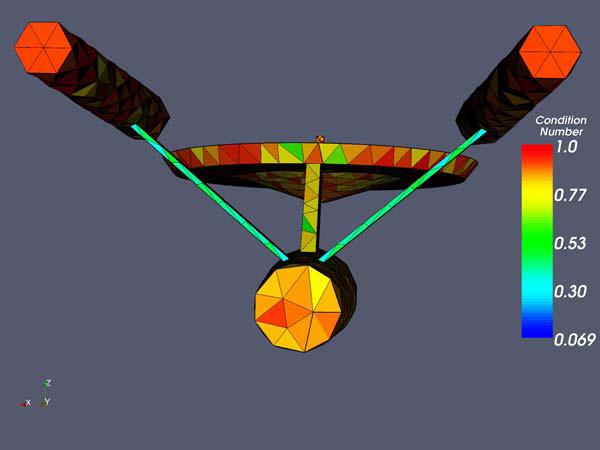
The initial mesh. The minimum modified condition number is 0.069 the mean is 0.82.

We have a higher resolution mesh to describe the boundary.

  cp ../../../data/geom/mesh/32/enterpriseL20.txt enterpriseBoundary.txt 

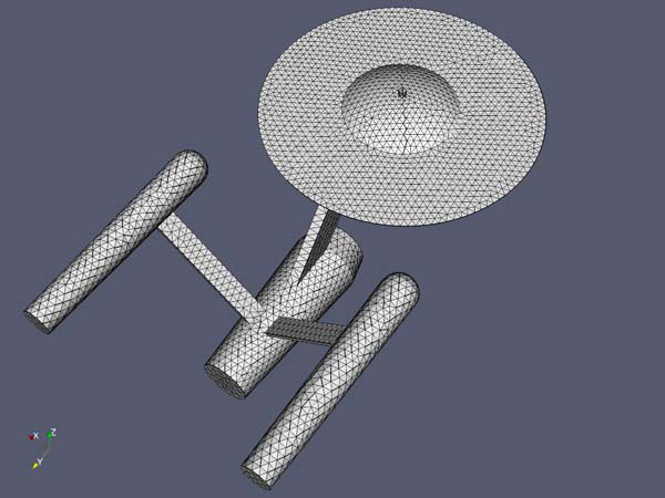
A higher resolution surface mesh of the Enterprise.

We apply apply one sweep of geometric optimization to the mesh. We optimize the modified condition number quality metric. First, we use an implicit description of the boundary. To optimize a boundary node, its position is first optimized in 3-D space and then projected back onto its closest point on the boundary. If the resulting change locally improves the quality of the mesh, it is accepted.

  optimization/geomOptBoundaryCondition3.exe -function=c enterpriseBoundary.txt enterprise.txt enterpriseImplicitSurface.txt 

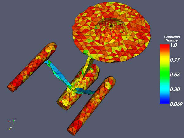
The mesh after optimization using the implicit surface method. The minimum modified condition number is 0.19 the mean is 0.85.

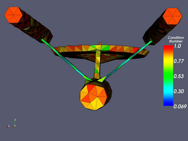
The mesh after optimization using the implicit surface method. View from the back.

We see that the optimization has improved the quality of the mesh elements. However, the result is not very satisfactory. The shape of the object has changed. The distortion is most pronounced on the thin rectangular beams and along the circular rim.

Next we try using a content constraint. That is, when moving boundary nodes the volume of the object remains constant.

  optimization/geomOptContentConstraint3.exe -function=c enterprise.txt enterpriseContentConstraint.txt 

The mesh after optimization using the content constraint method. The minimum modified condition number is 0.31 the mean is 0.87.

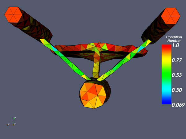
The mesh after optimization using the content constraint method. View from the back.

Again the optimization has improved the quality of the mesh elements. In this respect, it is more successful than with using the implicit boundary method. But again, the result is not very satisfactory. The shape of the object has been preserved along its its smooth surfaces, but it has been distorted near sharp edges in the model.

To rectify this problem, we utilize the edge features of the boundary mesh. We define any edge with a dihedral angle which deviates more than 0.5 from to be an edge feature. In the figure below we see that this choice is large enough to capture the edge features of the boundary mesh and small enough to not introduce spurious edge features. Intersecting edge features are corner features (shown in red).

  utility/extractFeatures32.exe -angle=0.5 enterpriseBoundary.txt enterpriseEdges.txt enterpriseCorners.txt 

The edge and corner features of the boundary mesh for a dihedral angle deviation of 0.5.

Now we optimize the mesh using the manifold with features approach to constrain the boundary nodes. In short, this means that for boundary nodes:

• Nodes on corner features cannot be moved.
• When nodes on edge features are moved, they must remain on that edge feature.
• When boundary nodes on surface features are moved, they must not cross edge features.

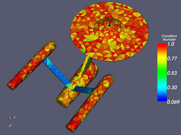
The mesh after optimization using the manifold with features approach. The minimum modified condition number is 0.10 the mean is 0.85.

The mesh after optimization using the manifold with features approach. View from the back.

We see that the optimization has not improved the quality of the elements as much as before, but the shape of the object has been accurately maintained.

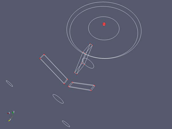
For this example, it is difficult to see how the mesh changed when using the manifold with features approach. One might ask whether the shape of the model was preserved because the nodes were moved well or whether they just were not moved. The following figures show the edges for the initial mesh in red and the edges for the optimized mesh in blue. They show that nodes on surface features were allowed to move along the surface and nodes on edge features were allowed to move along edge features.

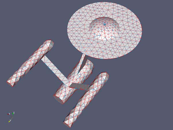
The edges of the initial mesh (in red) and the edges of the optimized mesh using the manifold with features approach (in blue).

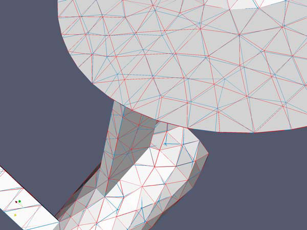
Close-up view.